목적
1. 이미지 데이터의 분류(classification)
2. 학습 데이터의 가공 방법
3. 학습의 조기종료 방법
4. 모델의 문제점 분석과 개선 전략
5. 학습 모델의 저장과 로드 사용
데이터셋
패션_엠니스트 | TensorFlow Datasets
이 페이지는 Cloud Translation API를 통해 번역되었습니다. 패션_엠니스트 컬렉션을 사용해 정리하기 내 환경설정을 기준으로 콘텐츠를 저장하고 분류하세요. Fashion-MNIST는 60,000개의 예제로 구성된
www.tensorflow.org
WxH=28x28 의 1채널 그레이 이미지로 60,000개의 학습용과 10,000개의 테스트용으로 구성
레벨 데이터는 아래와 같이 10개 구성
| 0 | T-shirt/top |
| 1 | Trouser |
| 2 | Pullover |
| 3 | Dress |
| 4 | Coat |
| 5 | Sandal |
| 6 | Shirt |
| 7 | Sneaker |
| 8 | Bag |
| 9 | Ankle boot |
1. 패키지 설치
|
pip install keras
pip install scikit-learn pip install pandas pip install numpy pip install seaborn |
2. 임포트
|
import numpy as np
import pandas as pd
import matplotlib.pyplot as plt
import seaborn as sns
import keras
from keras.datasets import fashion_mnist
from keras.models import Model, Sequential
from keras.layers import Dense, Dropout, Flatten
from keras.layers import Conv2D, AveragePooling2D, MaxPooling2D
from keras import optimizers, losses, metrics
from sklearn. import import confusion_matrix
|
3. 데이터셋 다운로드
|
(x_train, y_train), (x_test, y_test)= fashion_mnist.load_data()
|
x_train의 구조: (60000, 28, 28)
y_train의 구조 : (60000,)
x_test 의 구조 : (10000, 28, 28)
y_test 의 구조 : (10000,)
4. 학습용 데이터의 가공과 정규화
|
x_train = x_train.reshape((x_train.shape[0], 28, 28, 1)).astype("float32")
x_test = x_test.reshape((x_test.shape[0], 28, 28, 1)).astype("float32")
x_train /= 255 x_test /= 255 |
- reshape 의 이유는모델이 채널 데이터를 요구하기 때문 (Gray = 1 채널, Color = 3 채널)
(., 28, 28) -> [ [ 0, 23, 9, 8 ....] ....] (., 28, 28, 1) -> [ [ [0], [23], [9], [8] ....] ....] - reshape(-1, 1) 즉 2차원으로 변환은 손실함수 sparse_categorical_crossentropy 와 categorical_crossentropy 에서는 필요하지 않기 때문이다. ※ 회귀(Regression) 모델에서만 필요
- y_train / y_test 에는 [ 해당레벨, 해당레벨, .... ] 형태로 되어 있고 해당레벨은 0 ~ 9 의 값을 가진다.
- to_categorical (원-핫 인코딩 변환) 의 사용 유무
손실함수로 sparse_categorical_crossentropy 를 사용하는 경우 불필요 (내부적으로 정수레이블을 처리)
손실함수로 categorical_crossentropy 를 사용하는 경우 필요
from keras.utils import to_categorical
num_classes = 10one_hot_labels = to_categorical(original_labels, num_classes=num_classes)
5. 모델 정의
|
model = Sequential([
Conv2D(32, (3, 3), activation='relu', input_shape=(28, 28, 1)),
MaxPooling2D((2, 2)),
Conv2D(64, (3, 3), activation='relu'),
MaxPooling2D((2, 2)),
Flatten(),
Dense(128, activation='relu'),
Dropout(0.5),
Dense(10, activation='softmax') # 바이너리(2진) 분리시에는 sigmoid 를 사용
])
model.summary()
|
┏━━━━━━━━━━━━━━━━━━━━━━━━━━━━━━━━━┳━━━━━━━━━━━━━━━━━━━━━━━━┳━━━━━━━━━━━━━━━┓
┃ Layer (type)                    ┃ Output Shape           ┃       Param # ┃
┡━━━━━━━━━━━━━━━━━━━━━━━━━━━━━━━━━╇━━━━━━━━━━━━━━━━━━━━━━━━╇━━━━━━━━━━━━━━━┩
│ conv2d_4 (Conv2D)               │ (None, 26, 26, 32)     │           320 │
├─────────────────────────────────┼────────────────────────┼───────────────┤
│ max_pooling2d_4 (MaxPooling2D)  │ (None, 13, 13, 32)     │             0 │
├─────────────────────────────────┼────────────────────────┼───────────────┤
│ conv2d_5 (Conv2D)               │ (None, 11, 11, 64)     │        18,496 │
├─────────────────────────────────┼────────────────────────┼───────────────┤
│ max_pooling2d_5 (MaxPooling2D)  │ (None, 5, 5, 64)       │             0 │
├─────────────────────────────────┼────────────────────────┼───────────────┤
│ flatten_5 (Flatten)             │ (None, 1600)           │             0 │
├─────────────────────────────────┼────────────────────────┼───────────────┤
│ dense_10 (Dense)                │ (None, 128)            │       204,928 │
├─────────────────────────────────┼────────────────────────┼───────────────┤
│ dropout_2 (Dropout)             │ (None, 128)            │             0 │
├─────────────────────────────────┼────────────────────────┼───────────────┤
│ dense_11 (Dense)                │ (None, 10)             │         1,290 │
└─────────────────────────────────┴────────────────────────┴───────────────┘
6. 모델에 손실함수와 최적화 함수를 지정
|
model.compile(optimizer='adam', loss='sparse_categorical_crossentropy', metrics=['accuracy'])
|
※ 스페링을 기억하기 어려울 경우는 아래와 같이 사용 가능
|
model.compile(
optimizer=optimizers.Adam(),
loss=losses.SparseCategoricalCrossentropy(),
metrics=[metrics.SparseCategoricalAccuracy()]
)
|
7. 조기 종료 콜백 설정
|
early_stopping_callback = EarlyStopping(
monitor='val_loss', # 검증 손실을 모니터링 patience=3, # 3 에포크 동안 개선이 없으면 중단 restore_best_weights=True, # 최적의 가중치 복원 verbose=1 # 조기 종료 시 메시지 출력 ) |
8. 학습과 모델(파라미터 포함) 의 파일 저장
|
history = model.fit(x_train, y_train, epochs=10, batch_size=64, validation_split=0.2, callbacks=[early_stopping_callback])
k_es_model_path = 'keras_early_stopping_best_model.keras' keras_early_stopping_model.save(k_es_model_path, save_format='keras') |
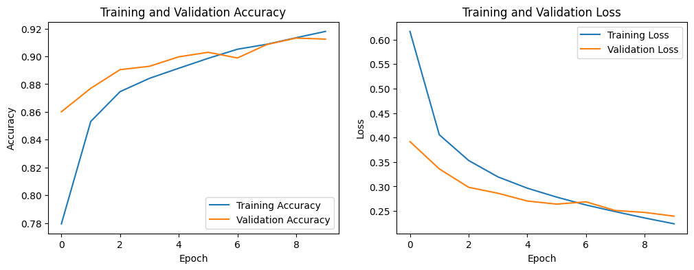
9. 학습시의 추이 그래프
|
plt.figure(figsize=(12, 4))
plt.subplot(1, 2, 1)
plt.plot(history.history['accuracy'], label='Training Accuracy')
plt.plot(history.history['val_accuracy'], label='Validation Accuracy')
plt.xlabel('Epoch')
plt.ylabel('Accuracy')
plt.legend()
plt.title('Training and Validation Accuracy')
plt.subplot(1, 2, 2)
plt.plot(history.history['loss'], label='Training Loss')
plt.plot(history.history['val_loss'], label='Validation Loss')
plt.xlabel('Epoch')
plt.ylabel('Loss')
plt.legend()
plt.title('Training and Validation Loss')
plt.show()
|
10. 학습 모델의 전반적인 성능
|
loss, accuracy = model.evaluate(x_test, y_test, verbose=0)
print(f'Test Loss: {loss:.4f}')
print(f'Test Accuracy: {accuracy:.4f}')
|
Test Loss: 0.2561
Test Accuracy: 0.9066
11. 클래스별 세부 성능 분석
|
from sklearn.metrics import classification_report, confusion_matrix
import numpy as np
import seaborn as sns
import matplotlib.pyplot as plt
# Predict probabilities for the test set
y_pred_probabilities = model.predict(x_test)
# Convert probabilities to class labels (e.g., the class with the highest probability)
y_pred = np.argmax(y_pred_probabilities, axis=1)
# Generate a classification report
print("\n--- Classification Report ---")
class_names = ['T-shirt/top', 'Trouser', 'Pullover', 'Dress', 'Coat', 'Sandal', 'Shirt', 'Sneaker', 'Bag', 'Ankle boot']
print(classification_report(y_test, y_pred, target_names=class_names))
# Generate and display the confusion matrix
print("\n--- Confusion Matrix ---")
cm = confusion_matrix(y_test, y_pred)
plt.figure(figsize=(10, 8))
sns.heatmap(cm, annot=True, fmt='d', cmap='Blues', xticklabels=class_names, yticklabels=class_names)
plt.xlabel('Predicted Label')
plt.ylabel('True Label')
plt.title('Confusion Matrix')
plt.show()
|
학습에 있어서 평가 항목 Accuracy 는 학습과 테스트에 사용되는 데이터의 구성에 따라 결과 값이 영향을 받는다.
예를 들면 한쪽 클래스만 편향된 학습데이터 구성이라면 아무리 Accuracy 가 높다해도 실제로 다른 클래스도 잘 분류한다고 볼 수 없다.
데이터셋에 특정 클래스(예: 정상 데이터)가 다른 클래스(예: 이상 데이터)보다 훨씬 많은 경우, 모델이 모든 것을 다수 클래스로만 예측해도 정확도는 높게 나올 수 있습니다. 하지만 이는 소수 클래스에 대해서는 전혀 예측을 못하는, 쓸모없는 모델일 수 있습니다. Precision, Recall, F1-Score는 각 클래스별 성능을 개별적으로 보여주기 때문에 이러한 불균형 데이터셋에서 모델의 진짜 성능을 평가하는 데 필수적입니다.

| precision(정밀도) | 사실로 답한 총수(TP + FP)중에 진짜사실의 판단수(TP) | 예) 암이라고 판정한 것 중 진짜 암의 비율 즉, 거짓 암판정(FP)을 줄이는데 중점 |
| recall(재현율) | 진짜사실의 총수(TP + FN)중에 진짜사실의 판단수(TP) | 예) 전체 진짜 암 환자중 실제 암 환자 판정 비율 즉, 진짜 암환자를 놓치지 않고 찾아내는데 중점 |
| f1-score | 정밀도와 재현율의 균형을 보여주는 지표 | 정밀도와 재현율이 불균형할 경우 F1-Score는 낮은 값을 가짐 |
| support | 각 클래스의 데이터 수 | 각각 1000개씩으로 균형 잡혀있다. |
--- Confusion Matrix ---
모델이 각 클래스를 어떻게 혼동하는지 시각적으로 상세하게 파악
행: 실제 클래스, 열: 예측 클래스

특히 Shirt 가 T-shirt/top 에 혼동되어 분류되었음을 알 수 있다.
12. 모델의 문제점 분석과 개선 전략
문제점 분석:
- 클래스 간 유사성:
'Shirt'는 'T-shirt/top' (티셔츠/상의)이나 'Pullover' (스웨터)와 같은 다른 의류 항목과 시각적으로 유사한 특징을 많이 공유할 수 있습니다. 예를 들어, 긴팔 셔츠와 긴팔 티셔츠, 또는 얇은 셔츠와 가벼운 풀오버 등은 형태나 질감에서 모델이 구분하기 어려울 수 있습니다. 혼동 행렬에서 'Shirt'가 'T-shirt/top' (151개)과 'Pullover' (65개)로 오분류되는 경향이 이 가설을 뒷받침합니다. - 클래스 내 다양성 (Intra-class Variance):
'Shirt'라는 카테고리 자체가 매우 다양한 스타일(드레스 셔츠, 캐주얼 셔츠, 블라우스 등)을 포함할 수 있습니다. 이 다양한 스타일들이 하나의 'Shirt'로 학습되기 때문에 모델이 공통된 특징을 학습하는 데 어려움을 겪을 수 있습니다. - 데이터 부족 또는 불균형 (품질):
비록 'support'는 각 클래스당 1000개로 균형 잡혀 있지만, 'Shirt' 이미지의 품질이 다른 클래스에 비해 낮거나, 'Shirt' 클래스 내의 다양한 스타일을 대표하기에 데이터의 다양성이 부족할 수 있습니다.
대처 방안 (개선 전략):
- 데이터 증강 (Data Augmentation):
'Shirt' 클래스 이미지에 대해 회전, 확대/축소, 좌우 반전, 밝기 조절 등 다양한 변형을 주어 데이터셋의 양을 늘리고 모델이 더 일반적인 특징을 학습하도록 돕습니다. - 오류 분석 및 데이터 클리닝 (Error Analysis & Data Cleaning):
모델이 'Shirt'를 'T-shirt/top'이나 'Pullover'로 잘못 분류한 이미지들을 직접 살펴봅니다. 왜 모델이 혼동했는지 시각적으로 파악하면 문제 해결에 도움이 됩니다. 혹시 잘못 라벨링된 이미지는 없는지 확인합니다.
특히 'Shirt' 클래스 내에서 대표성이 부족한 스타일이 있다면, 해당 스타일의 이미지를 추가 확보하는 것을 고려합니다. - 모델 아키텍처 개선 (Model Architecture Improvement):
더 깊거나 넓은 네트워크: 현재 모델보다 더 많은 계층(layer)이나 더 많은 필터(filter)를 사용하여 모델의 표현력을 높여봅니다.
전이 학습 (Transfer Learning): ImageNet과 같이 대규모 이미지 데이터셋으로 사전 학습된 모델(예: ResNet, VGG 등)을 가져와 Fashion MNIST 데이터에 맞게 미세 조정(fine-tuning)하는 것을 고려할 수 있습니다. 이는 복잡한 특징을 효과적으로 학습하는 데 큰 도움이 됩니다. - 클래스 가중치 적용 (Class Weighting):
'Shirt' 클래스의 예측 오류에 더 높은 가중치를 부여하여, 모델이 학습 시 'Shirt' 클래스를 더 중요하게 다루도록 설정할 수 있습니다. 이는 model.fit() 함수의 class_weight 인자를 통해 구현할 수 있습니다. - 특징 학습 강화:
'Shirt'와 다른 유사 클래스를 구분하는 데 도움이 되는 특징(예: 칼라, 소매 길이, 단추 여부 등)을 모델이 더 잘 학습하도록 유도하는 방안을 고민할 수 있습니다. 경우에 따라서는 이러한 특징들을 수동으로 추가하거나, 모델이 더 세부적인 특징을 포착하도록 하는 방법을 고려할 수도 있습니다.
이러한 방법들을 조합하여 적용함으로써 'Shirt' 클래스의 분류 성능을 개선할 수 있습니다. 가장 먼저 데이터 증강과 오류 분석을 통해 문제의 근본 원인을 파악하는 것이 좋습니다.
13. 학습된 모델 화일을 로드하여 추론
|
# 학습 후 저장된 Keras 모델 파일을 다시 불러와 `loaded_keras_model` 변수에 할당합니다.
loaded_keras_model = keras.models.load_model('keras_early_stopping_best_model.keras')
# 여기서 x_test는 테스트 데이터입니다. 형태는 [ [ [ ] [ ] .... ] ...] (28, 28, 1) x 5 입니다. unknown_data = x_test[:5]
unknown_predictions_probabilities = loaded_keras_model.predict(unknown_data)
# 확률을 클래스 레이블로 변환 (가장 높은 확률을 가진 클래스 선택)
unknown_predicted_labels = np.argmax(unknown_predictions_probabilities, axis=1) class_names = ['T-shirt/top', 'Trouser', 'Pullover', 'Dress', 'Coat', 'Sandal', 'Shirt', 'Sneaker', 'Bag', 'Ankle boot'] for i in range(len(unknown_data)): predicted_label_idx = unknown_predicted_labels[i] print(f"샘플 {i+1}: 예측='{class_names[predicted_label_idx]}' (ID: {predicted_label_idx})") |
'data science > Artificial Intelligence' 카테고리의 다른 글
| Token과 Embedding의 원리 쉽게 이해하기 (0) | 2026.06.10 |
|---|---|
| [deep learning] 2. Fashion MNist (pytorch 버젼) (0) | 2026.02.07 |
| [deep learning] 1. Combined Cycle Power Plant (keras 버젼) (0) | 2026.02.06 |
| Transformer (GPT) 가장 쉽게 이해하기 - Part 2 (0) | 2025.10.26 |
| Transformer (GPT) 가장 쉽게 이해하기 - Part 1 (0) | 2025.10.19 |